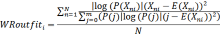
Gao et al. (2025) "propose a new person-fit statistic, WR, specifically designed for polytomous items in CDMs" [Cognitive Diagnostic Models]. As implemented in Winsteps, the fundamental equation is:
![]()
where i is item i, n=1 to N are the persons, Xni is the observation of category j of the rating scale, j=0,m. |log(P(Xni=j)| is the absolute value of the probability that Xni is j. E(Xni) is the expected value of Xni. There is a similar computation for each person n, where i=1 to L are the items.
When WRFIT=Yes, Winsteps reports the WR-GHWZ statistic. Gao et al. (2025) do not report WR-GHWZ directly. Instead they report significance tests based on bootstrap resampling. Bootstrap resampling can be done in Winsteps using SIMUL=.
WR-GHWZ is the squared residual weighted by the log-probability of the observation. This same weighting can be applied to the usual Infit and Outfit mean-square statistics: Computation of OUTFIT and INFIT Statistics. When WRFIT=Yes, WR-Infit mean-square and WR-Outfit mean-square are also reported.
![]()
Gao X., Hou M., Wang F., Zhou J, (2025) A new person‑fit statistic for the detection of aberrant responses in polytomous cognitive diagnostic models. Behavior Research Methods 57:138. https://doi.org/10.3758/s13428-025-02659-6
Example: Table 6 for the data sets in Polytomous Mean-Square Fit Statistics and Dichotomous Infit and Outfit Mean-Square Fit Statistics are shown below. Gao et al.(2025) report that "Overall, WR proved to be an effective tool for detecting person misfit in polytomous scoring CDMs." They investigated "highly competent examinees respond[ing] incorrectly to simple items in a unique and creative way", and "cheating where low-ability examinees use various methods, such as cheating and plagiarism, to provide correct answers to difficult items". These are "noisy outliers" in the polytomous Table below.
POLYTOMOUS MISFIT STATISTICS
-------------------------------------------------------------------------------
|INFIT OUTFIT| GHWZ INFIT OUTFIT| |
|MNSQ |MNSQ | WR WR-MS WR-MS| PERSON |
+------+------+-------------------+-------------------------------------------|
| 8.30 | 9.79 |4.5905 20.2 25.1 | 00000000003333333333 extreme reversal |
| 5.14 | 6.07 |3.4927 11.7 14.9 | 03030303030303030303 extreme flip-flop |
| 4.00 | 5.58 |3.1322 9.41 13.9 | 00111111112222222233 Guttman reversal |
| 3.62 | 4.61 |2.8802 7.96 10.8 | 01230123012301230123 rotate categories |
| 2.11 | 4.14 |1.1708 1.97 3.62 | 22222222223333333333 high reversal |
| 2.99 | 3.59 |2.5150 6.28 7.63 | 03202002101113311002 random responses |
| 2.56 | 3.20 |1.8663 3.34 4.36 | 11111111112222222222 central reversal |
| 1.75 | 2.02 |1.5010 2.16 2.59 | 11111122233222111111 folded pattern |
| 1.50 | 1.96 |1.4281 1.96 2.65 | 12121212121212121212 central flip-flop |
| 1.49 | 1.40 |1.3055 1.64 1.51 | 33133330232300101000 noisy progression |
| 1.37 | 1.20 |1.0356 1.03 .85 | 33333333330000000000 extreme categories |
| 1.25 | 1.09 |1.0466 1.08 .87 | 33233332212333000000 erratic transitions |
| .94 | 1.22 |1.4783 2.10 2.87 | 32222222201111111130 noisy outliers |
| .85 | 1.21 | .8364 .72 .98 | 22222222222222222222 one category |
| 1.06 | .97 | .9185 .81 .68 | 33333331122300000000 modelled |
| .98 | 1.04 | .9119 .80 .90 | 31332332321220000000 modelled |
| 1.03 | 1.00 | .8652 .72 .68 | 33333331110010200001 modelled |
| .98 | .99 | .8113 .64 .62 | 33333132210000001011 modelled |
| .80 | .77 | .6819 .45 .41 | 33333333221100000000 high discrimination |
| .52 | .54 | .5558 .30 .29 | 32323232121212101010 tight progression |
| .31 | .36 | .3513 .12 .13 | 33333222221111100000 most likely |
| .25 | .34 | .4018 .15 .21 | 22222222221111111111 2 central categories |
| .21 | .26 | .3390 .11 .13 | 32222222221111111110 low discrimination |
| .24 | .24 | .2863 .12 .11 | 33333333332222222222 high (low) categories|
| .18 | .22 | .2947 .08 .09 | 33222222221111111100 most expected |
| .16 | .20 | .2687 .08 .08 | 33333322222222211111 only 3 categories |
+------+------+-------------------+-------------------------------------------|
DICHOTOMOUS MISFIT STATISTICS
-----------------------------------------------------------------------------
|INFIT|OUTFIT| GHWZ INFIT OUTFIT| |
|MNSQ |MNSQ | WR WR-MS WR-MS| PERSON |
+-----+------+-------------------+------------------------------------------|
|4.75 |8.05 |1.1913 7.85 8.81 | 0000000011111111 Miscode |
|2.37 |3.31 | .7900 3.45 3.58 | 1010101010101010 Response set/Miskey |
|1.76 |1.32 | .5620 1.75 1.56 | 1111000011110000 Special knowledge |
| .87 |1.73 | .4636 1.19 1.67 | 0111111110000000 Carelessness/Sleeping |
| .87 |1.73 | .4636 1.19 1.67 | 1111111000000001 Lucky Guessing |
|1.59 |1.45 | .5653 1.77 1.59 | 1110101010101000 low discrimination |
|1.15 | .91 | .4406 1.07 .95 | 1111010110010000 Imputed outliers |
|1.13 | .95 | .4440 1.09 .99 | 1110110110100000 Modelled/Ideal |
| .68 | .45 | .2734 .41 .40 | 1111110101000000 high discrimination |
| .50 | .34 -| .2026 .23 .23 | 1111111010000000 very high discrimination|
| .41 | .29 -| .1593 .14 .14 | 1111111100000000 Guttman/Deterministic |
+-----+------+-------------------+------------------------------------------|
TITLE='POLYTOMOUS MISFIT STATISTICS
WRFIT=Yes
NI=20
ITEM1=1 ; include response strings in person name
name1=1
namlen=43
CODES=0123
ptbis=no ; compute point-measure correlation
INUMB=YES ; no item labels
TFILE=*
6 ; Table 6 - persons in fit order
18 ; table 18 - persons in entry order
*
IAFILE=* ; item anchor values - uniform
1 -1.9
2 -1.7
3 -1.5
4 -1.3
5 -1.1
6 -0.9
7 -0.7
8 -0.5
9 -0.3
10 -0.1
11 0.1
12 0.3
13 0.5
14 0.7
15 0.9
16 1.1
17 1.3
18 1.5
19 1.7
20 1.9
*
SAFILE=* ; step anchor values
0 0
1 -1
2 0
3 1
*
&end
33333132210000001011 modelled
31332332321220000000 modelled
33333331122300000000 modelled
33333331110010200001 modelled
33222222221111111100 most expected
33333222221111100000 most likely
33333333221100000000 high discrimination
32222222221111111110 low discrimination
32323232121212101010 tight progression
33333333332222222222 high (low) categories
22222222221111111111 2 central categories
33333322222222211111 only 3 categories
32222222201111111130 noisy outliers
33233332212333000000 erratic transitions
33333333330000000000 extreme categories
33133330232300101000 noisy progression
22222222222222222222 one category
12121212121212121212 central flip-flop
03202002101113311002 random responses
01230123012301230123 rotate categories
03030303030303030303 extreme flip-flop
11111122233222111111 folded pattern
22222222223333333333 high reversal
11111111112222222222 central reversal
00111111112222222233 Guttman reversal
00000000003333333333 extreme reversal
Title = DICHOTOMOUS MISFIT STATISTICS
wrfit=yes
ni=16
item1=1
name1=1
namelength=41
codes=01
ptbiserial = measure
iafile=*
1 1
2 2
3 3
4 4
5 5
6 6
7 7
8 8
9 9
10 10
11 11
12 12
13 13
14 14
15 15
16 16
*
uascale = 2.4
tfile=*
6 ; Table 6 - persons in misfit order
*
&end
END LABELS
1110110110100000 Modelled/Ideal
1111111100000000 Guttman/Deterministic
0000000011111111 Miscode
0111111110000000 Carelessness/Sleeping
1111111000000001 Lucky Guessing
1010101010101010 Response set/Miskey
1111000011110000 Special knowledge
1111010110010000 Imputed outliers
1110101010101000 low discrimination
1111110101000000 high discrimination
1111111010000000 very high discrimination